When managing large-scale data lakes with Microsoft Fabric, performance optimisation becomes crucial. One effective technique to achieve better performance is Delta Lake partitioning. Partitioning can significantly enhance query performance, reduce computational costs, and improve data management efficiency within Microsoft Fabric environments.
In this blog post, we will explore what Delta Lake partitioning is, how it works, and why it matters. We’ll also discuss best practices for creating effective partitions, common pitfalls to avoid, and practical examples demonstrating the real-world impacts of partitioning on query performance.
What is Delta Lake Partitioning?
Before we can understand what partitioning in Delta Lake actually is, we need to understand a little bit more about delta tables in general. In the next paragraph I will introduce the concept of a delta table, after that we will look at how we can optimise them using partitions.
What is a delta table?
A delta table is a storage construct within the open source Delta Lake project. It is used by Microsoft Fabric and other platforms as the go-to storage layer for structured, tabular data.
A data lake consists of file storage. One of the more popular formats for data lake storage is the parquet file. This is a file format that is highly optimised for analytical processing. There are issues, however. For starters, it is impossible to change data in a parquet file – they are immutable. Also, it’s not possible to run ACID transactions on a parquet file. ACID stands for atomicity, consistency, isolation, durability, and describes properties of a database transaction to guarantee data validity.
In a traditional relational database such as SQL Server, transactions ensure the validity of your data. In a data lake, this is not possible using just parquet files.
So, a delta table is basically a parquet file on steroids! It is file storage (parquet) with table-like features such as transactions and the possibility to run insert/update/delete statements against your data. In short, it transforms your data lake into a delta lake that can easily process your data.
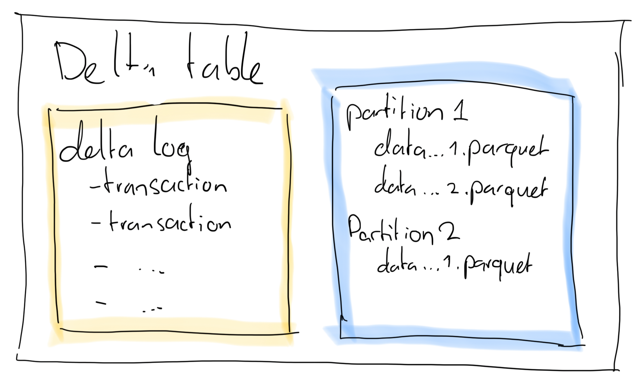
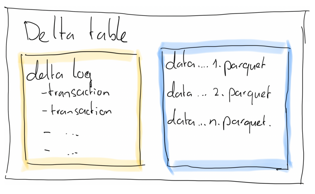
The delta table consists of at least 1 parquet file holding the physical data of the table, and a transaction log that contains JSON-documents describing transactions that have run on the table.
Delta Table Partitioning
While a delta table on your data lake consists of at least 1 parquet file, in practice there can be many files. This can happen due to a large data volume, in which case it might be efficient to split up a large file in chunks. It may also happen as a result of frequent updates and inserts. Remember, a parquet file is immutable and therefore you need to write new files in order to update or insert data into a delta table.
Now if data volumes grow, it might be wise to start partitioning your delta tables. You, as the developer or data engineer, are in charge of doing that. Nobody, not Microsoft Fabric, not Spark, not Delta Lake, is automatically partitioning your data.
So, what is delta lake partitioning exactly?
Delta Lake partitioning is essentially a way of organising a large table into more manageable, logical chunks. Instead of forcing your queries to search through every row of data, partitioning by a specific column (for example, date) ensures that the Spark engine only scans the subset of data you actually need.
This structure not only trims down query times, but also helps keep costs under control in Microsoft Fabric, since fewer resources are spent scanning irrelevant information. In practice, it’s a simple concept that can have a major impact on the efficiency and scalability of your data lakehouse environment.
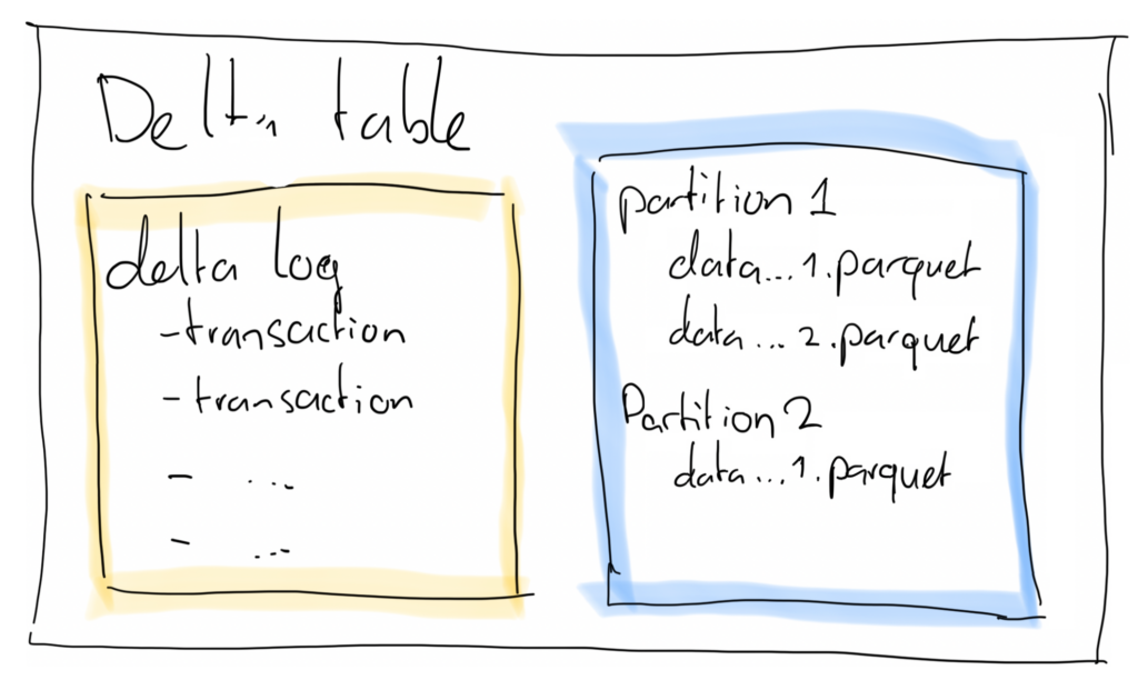
The way this works is by choosing a column (or columns) to split up the parquet files. So instead of having 1..n files in your delta table, you now have a folder per partition (be it Date, Region, or any other column you use to partition by) so that you have 1..n files per partition. Queries that filter on a partition column can now use partition elimination to find results much faster.
How to Optimise Delta Tables using Partitioning in Microsoft Fabric for Faster Queries
A delta table can contain many rows. I have seen them in the billions of rows already, both in practice at client projects as well as in my demo showing 4 billion rows in DirectLake in Power BI.
Now let’s say your dataset is huge. If you are running analyses on this data, you might be executing queries, filtering data, etc. Or, you might be building a Power BI DirectLake model on top of this delta table. In that case, Power BI will be executing queries against your delta tables.
If the table is large, that could lead to bad performance. If the engine must search through many millions of rows to find the answer, it could take a lot of time.
This is where partitioning comes into play. If you partition a table, it will be split up into multiple files, according to the column you use to partition the table by.
Let’s assume we have a column called ‘Date’ in our table, and we partition by date, then under the hood the table will be split into 1 table per date in your data. If you then run a query against this table that filters on the date column (or any other partitioned column), the engine doesn’t scan all data, but only the files that contain that particular date (or dates). That is much faster!
How to Create Partitions in Delta Lake?
Creating partitions in a delta table is done during the creation of the table. It is not possible to add partitions to a table after it is already created. So be careful and think through your scenario before creating a table. If you must change the partitioning of an existing table, you should:
- Create a new table with the new partitioning
- Copy data from the old table to the new table
- Remove the old table
- Rename the new table to the old table name
Creating a partition in your table is quite easy. In PySpark, I usually do the following:
DeltaTable.create(spark) \
    .tableName("gold_facttaxidata_PartitionDateTaxitype") \
    .addColumn("PickupDate", "DATE") \
    .addColumn("PickUpTime", "STRING") \
    .addColumn("DropoffDate", "DATE") \
    .addColumn("DropoffTime", "STRING") \
    .addColumn("PickupLocationId", "INT") \
    .addColumn("DropoffLocationId", "INT") \
    .addColumn("TaxiTypeId", "INT") \
    .addColumn("PassengerCount", "INT") \
    .addColumn("TripDistance", "DOUBLE") \
    .addColumn("FareAmount", "DOUBLE") \
    .addColumn("SurchargeAmount", "DOUBLE") \
    .addColumn("MTATaxAmount", "DOUBLE") \
    .addColumn("TipAmount", "DOUBLE") \
    .addColumn("TollsAmount", "DOUBLE") \
    .addColumn("ExtraAmount", "DOUBLE") \
    .addColumn("EhailFeeAmount", "DOUBLE") \
    .addColumn("AirportFeeAmount", "DOUBLE") \
    .addColumn("CongestionSurchargeAmount", "DOUBLE") \
    .addColumn("ImprovementSurchargeAmount", "DOUBLE") \
    .addColumn("_PickupYear", "INT", generatedAlwaysAs="YEAR(PickupDate)") \
    .addColumn("_PickupMonth", "INT", generatedAlwaysAs="MONTH(PickupDate)") \
    .partitionedBy("PickupDate", "TaxiTypeId") \
    .execute()
On line 24 you see that the partitioning is defined, in this case on PickupDate and TaxiTypeId. That means that physically, this table is split into a folder hierarchy looking something like “TableName/2025-03-21/1/data.parquet”. There are folders for PickupDate (i.e. 2025-03-21) and TaxiTypeId (i.e. 1). If your queries reference these columns in filters, the partition elimination will make sure only the parquet files in those folders will be searched. This will probably bring query time down.
Choosing the Right Columns for Delta Lake Partitioning
Using delta lake partitioning is not a silver bullet. If it’s used on the wrong columns, it can negatively impact performance instead of improving it.
The reason is simple. If you partition by a column that is almost never used in the filters, the engine must go through all the files (for all the partitions!) in order to find your data. This introduces overhead to the calculations. Without partitions, there would have been less files to go through.
If you select columns that you often filter by, such as date, company, product, or whatever, that might make most of your queries a lot faster.
Also, keep in mind that for smaller tables partitioning is usually not needed. Partitioning a small table might result in overhead compute usage when you start splitting into partitions that are too small. Spark is quite comfortable reading large parquet files, so there is an optimum!
Testing the Fabric Delta Partitions
In order to test our partitioning, let’s see how some trial queries perform. For one of my presentations earlier this year, I had to create a massive dataset. To do so, I downloaded the New York City taxi data from their website. It contains almost 4 billion (as of writing) taxi rides from 2009 to today.
I prepared all of this data into one massive delta table, and duplicated that table to a version with and one without partitioning. Then, we can look at how some queries perform when we run them against the two test tables.
Tip: run EXPLAIN in your SQL cell to see the query plan. For example:
%%sql
--partitioned
EXPLAIN
SELECT COUNT(*) AS total_trips
FROM gold_facttaxidata_notoptimised
WHERE PickupDate = '2020-01-01';
== Physical Plan == AdaptiveSparkPlan isFinalPlan=false +- HashAggregate(keys=[], functions=[count(1)]) +- Exchange SinglePartition, ENSURE_REQUIREMENTS, [plan_id=517] +- HashAggregate(keys=[], functions=[partial_count(1)]) +- Project +- Filter (isnotnull(PickupDate#786) AND (PickupDate#786 = 2020-01-01)) +- FileScan parquet spark_catalog.gold.gold_facttaxidata_notoptimised[PickupDate#786] Batched: true, DataFilters: [isnotnull(PickupDate#786), (PickupDate#786 = 2020-01-01)], Format: Parquet, Location: PreparedDeltaFileIndex(1 paths)[abfss://46d598b5-2ee2-42d4-aeb6-cad92ea22af3@onelake.dfs.fabric.m…, PartitionFilters: [], PushedFilters: [IsNotNull(PickupDate), EqualTo(PickupDate,2020-01-01)], ReadSchema: struct<PickupDate:date>
%%sql
--partitioned
EXPLAIN
SELECT COUNT(*) AS total_trips
FROM gold_facttaxidata_partitiondatetaxitype
WHERE PickupDate = '2020-01-01';
== Physical Plan == AdaptiveSparkPlan isFinalPlan=false +- HashAggregate(keys=[], functions=[count(1)]) +- Exchange SinglePartition, ENSURE_REQUIREMENTS, [plan_id=795] +- HashAggregate(keys=[], functions=[partial_count(1)]) +- Project +- FileScan parquet spark_catalog.gold.gold_facttaxidata_partitiondatetaxitype[PickupDate#1430,TaxiTypeId#1436] Batched: true, DataFilters: [], Format: Parquet, Location: PreparedDeltaFileIndex(1 paths)[abfss://46d598b5-2ee2-42d4-aeb6-cad92ea22af3@onelake.dfs.fabric.m…, PartitionFilters: [isnotnull(PickupDate#1430), (PickupDate#1430 = 2020-01-01)], PushedFilters: [], ReadSchema: struct<>
In bold and underlined, I have highlighted the differences you can see in the query plans for both queries. As you can clearly see, the query against optimised table includes a partition filter that will help the engine to minimise the data that has to be read.
Let’s see how different sample queries perform in an indexed vs unindexed table.
Before each test, I run “spark.catalog.clearCache()” in order to clear the cache.
Test case 1: Filter Query on Partition Columns
%%sql
--partitioned
SELECT COUNT(*) AS total_trips
FROM gold_facttaxidata_notoptimised
WHERE PickupDate = '2020-01-01';
Not optimised table: 2.790 seconds
Indexed table: 1.483 seconds
%%sql
--not optimised
SELECT COUNT(*) AS total_trips
FROM gold_facttaxidata_notoptimised
WHERE PickupDate >= '2020-01-01' and PickupDate <= '2020-12-31';
Not optimised table: 6.160 seconds
Indexed table: 11.729 seconds
Here something interesting becomes visible. Since we’ve partitioned our table on PickupDate, as long as we filter our query on a single data the performance improves. As you can see from the first sample, the indexed table is about twice as fast as the not optimised table.
However, once we start looking at (large) ranges of dates, such as a whole year, the performance improvement gets completely undone by the additional overhead the partitioning introduces. The unoptimised table is almost twice as fast as the indexed table.
The reason for this is simple. In the indexed table, the engine needs to read data from 366 (leap year!) files in order to find the number of rows for 2020. The overhead of reading all these files is what makes the query run twice as long as the same query against the regular table.
This is what I wrote earlier: sometimes it’s better to not index, if the result is a query that needs to read a lot of small files.
Test case 2: Aggregation Query Grouped by Partition Column
%%sql
SELECT PickupDate, COUNT(*) AS trip_count, AVG(FareAmount) AS avg_fare
FROM gold_facttaxidata_notoptimised
WHERE PickupDate >= '2020-01-01' AND PickupDate <= '2020-01-31'
GROUP BY PickupDate
ORDER BY PickupDate ASC
Not optimised table: 3.438 seconds
Indexed table: 3.538 seconds
This was a difficult one for the regular table as it had to scan all a lot of data. The same applies to the indexed table, but because that one had to traverse through 31 partitions it was a little bit slower than the unoptimised version!
Let’s filter for just three dates (2020-01-01 -> 2020-01-03) then the results become:
Not optimised table: 2.268 seconds
Indexed table: 1.417 seconds
Test case 3: Full table scan
SELECT COUNT(*) AS total_trips
FROM gold_facttaxidata_PartitionDateTaxitype;
Not optimised table: 1.644 seconds
Optimised table: 2.319 seconds
And again I’m the victim of a too granular approach to partitioning. As you can see, the full table scan to find the total number of rows in the table (3,867,399,283) is faster when not using partitions. This is likely due to the large number of days in the dataset, that spans from 2009 until 2024.
Conclusion
Delta lake partitioning can greatly improve query performance within your Microsoft Fabric environment, provided you carefully select the right columns to partition on. As demonstrated through our testing scenarios, partitioning isn’t always beneficial; excessive or improperly selected partitions can introduce performance overhead and degrade query speed. It’s essential to analyse query patterns and data usage carefully before deciding on a partitioning strategy. Ultimately, understanding and applying partitioning best practices will help you create optimised, scalable, and cost-effective Delta Lake tables, therefore improving the performance of you Microsoft Fabric data platform while lowering the costs.
1 thought on “Delta Lake Partitioning for Microsoft Fabric”